Alexander Lonin, Team Lead of polygonal modeling, Ph.D., presents an overview of the polygonal mesh topology operations, enhancements, new functionality, and plans for further polygonal modeling capability development.
Most geometric algorithms need more input data than just a mesh defined as a set of triangles. For example, consider how a mesh is converted from the STL format. Such a mesh is good only for visualization and calculating its area. For anything else, we need some topological structure. It is the foundation of polygonal modeling.
This structure contains two key components. The first is the representation of the mesh topology, which defines the relationships between vertices, edges, and polygons. The topology representation should support not only triangles but also polygons with an arbitrary number of sides (facets). The topology engine also performs some basic operations such as ordered traversal through the facets adjacent to the selected one; ordered traversal of the vertex fan; edge collapse; adding a vertex; edge flipping, and some others.
As a rule, we need the mesh not as a single entity, but as logically grouped facet clusters. Therefore, the second component of topology representation is meshing segmentation. A segmented mesh representation is similar to that of the conventional B-rep: faces, contours, and edges. The difference is that the faces are connected groups of facets, and the edges are sequences of the mesh edges. Similar to the mesh topology, there are some basic operations to handle the segmented mesh representation: various traversals of adjacent segments; new segmentation or re-segmentation with a set of edges or facets; merging of one or more segments; boundary facet swaps, and so on.
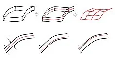
The figure shows an example of re-segmentation. Each segment is highlighted in a different color. The mesh is divided into segments by the yellow polyline. The second image is the result of such segmentation.
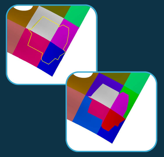
Figure 1
Each topology element also contains an abstract attribute: a number, vector, surface, or arbitrary data structure.
At first glance, all that above is well-known and easy to implement. However, an extensive range of algorithms built on basic operations is required. Their implementation is challenging and takes a lot of effort. Also, note that the topology representation should be up-to-date and valid at each step of each algorithm. In this way, we create a powerful, universal tool, and a foundation for solving any polygonal modeling problems. At the moment our polygonal modeling products are completely independent. We do not use any third-party or open-source solutions.
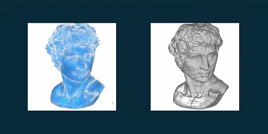
Now let us talk about the results obtained from such a comprehensive approach. Globally, all the available functionality is improved, mostly in terms of performance. The basic mesh healing operations are now reduced to topology creation. The healing eliminates the most obvious issues: duplicated vertices, degenerate or duplicated triangles, and non-consistent normal vectors. Any non-manifolds are also detected. The Boolean and 3D convex hull operations have been accelerated by x30...40. The larger the mesh, the greater the performance gain. Such operations as the detection of open boundaries or a boundary of a group of adjacent facets are now almost trivial. The figure shows the healing of a mesh with non-consistent normal vectors. In the first image, each triangle is inverted with respect to its neighboring triangles, In the second image, the mesh is healed.
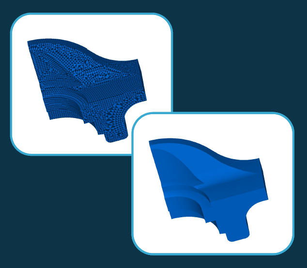
Figure 2
The new functionality includes the addition of 2D convex hull, mesh simplification, parameterization, and fitting NURBS and analytical surfaces to a group of polygons.
This figure shows that all the triangulation points are projected onto the plane. The convex hull is highlighted in blue. If the convex hull is available, we can construct the minimum bounding box.
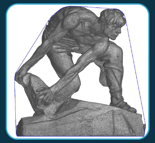
Figure 3
There are two mesh simplification options: reducing the number of triangles to the given value or accuracy. It is also possible to build a set of simplified meshes with various levels of detail. The simplification process is a sequence of edge collapses (one of the basic operations mentioned above). Some edge collapses are rejected, e.g., if the collapse results in the stitching of two triangles by their two edges, closing an open contour, etc. This maintains the integrity of the polygonal topology. If the polygonal model was a disk, it would remain a disk. If it had n contours or n handles, these numbers would not change.
The figures clearly show meshes with different levels of detail. For example, in the last image, the baby hippopotamus is simplified into a tetrahedron. Any further simplification is impossible without breaking its topological properties.
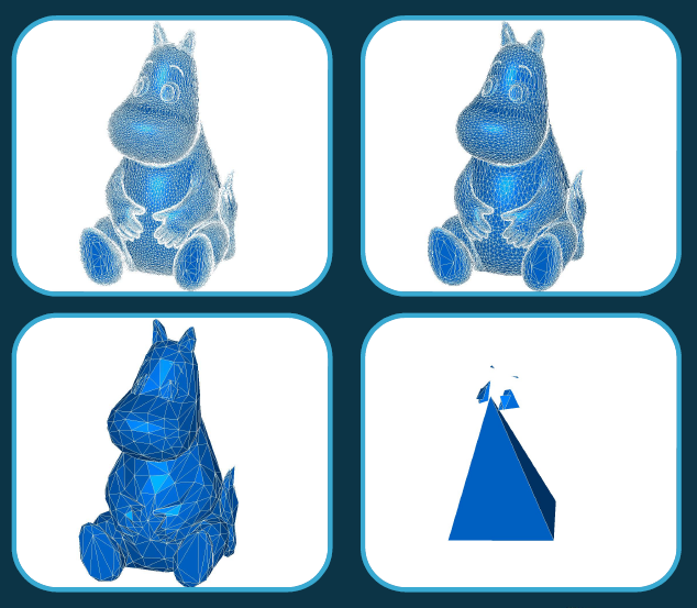
Figure 4
This is another example of the mesh simplification applied to a more complex topology.
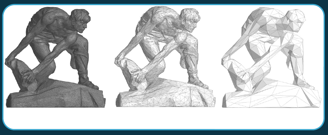
Figure 5
Although mesh parameterization is not yet available in the API, it is one of the key mesh processing tools. Let us analyze this using the open-source Napoleon face model.
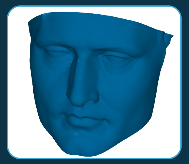
Figure 6
To put it simply, there are two parameterization options: free boundary and fixed boundary. Parametrization means the mapping of the mesh to the plane. The free boundary parametrization is the most general case with the highest computational costs. The algorithm generates 2D coordinates for each vertex of the mesh. It should be similar to a disk topologically. The following figure is generated by the algorithm.
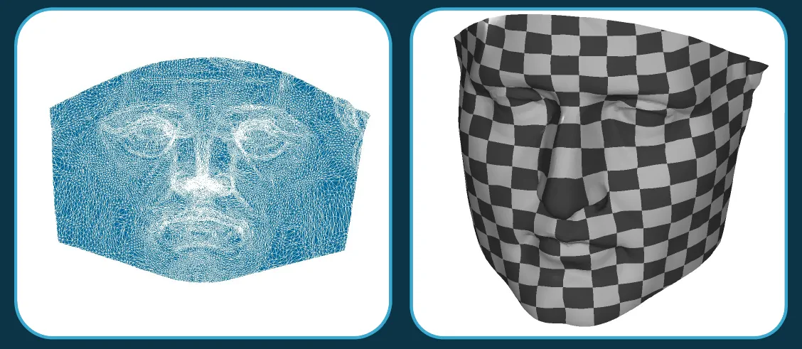
Figure 7
The left image is the face mapped on the plane. The best-known application of mesh parameterization is applying the textures to a complex surface. If we draw a regular rectangular mesh in 2D, in 3D it will look like the right image.
The fixed boundary parametrization is a simpler option. The 2D coordinates of the boundary vertices are specified by a certain rule, and the coordinates for the internal vertices are calculated. In the general case where no additional information is available, we can use the mapping to a circle. The left image is the face mapped to the circle, the 3D image is on the right.
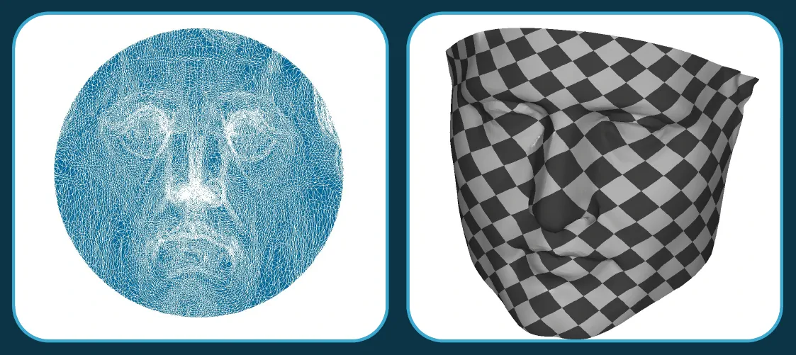
Figure 8
There can be some a priori knowledge of the mesh. For instance, in this case, the open boundary has four corners so the face can be mapped to a rectangle. Technically, this is the preferred option. The result is shown in the figure.
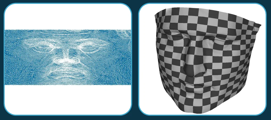
Figure 9
However, this approach has certain limitations. Let us try a more complicated mesh: the Stanford Rabbit. The left image is its mapping to a circle. The parametrization is extremely inconsistent: the bottom squares are small while the top ones are large. We need a new approach.
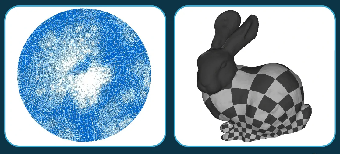
Figure 10
For NURBS surface fitting, the knot vector can be generated automatically. The inputs are the set of triangles, spline order, max number of spline control points, smoothing factor, and the expected fitting accuracy. The NURBS surface fitting is based on mesh parameterization. The parametrization produces 2D coordinates of the vertices. With these coordinates, we can approximate the surface.
The figure shows the results of several parameterization strategies.
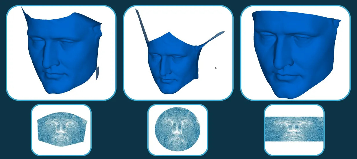
Figure 11
On the left is the most general open boundary parameterization. The surface matches the mesh well where the mesh is present, and deviates in a certain way where there is no mesh. Naturally, mapping to a circle is the least desirable case. Having some a priori information about the mesh provides better results.
The next image shows the control points of the resulting surface.
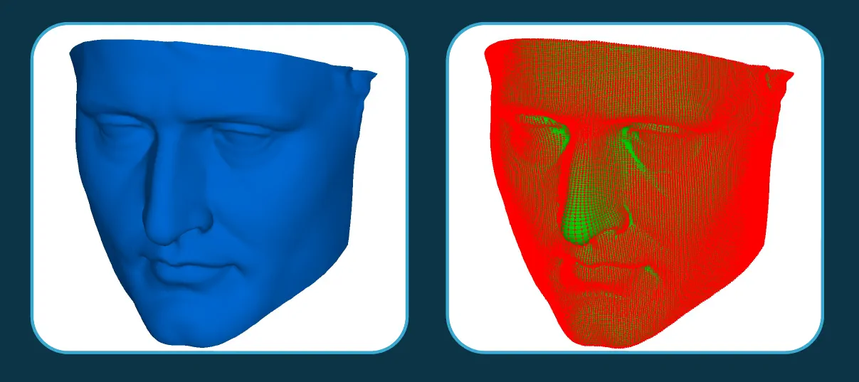
Figure 12
The following image shows the effects of the smoothing factor. The factor decreases from left to right.
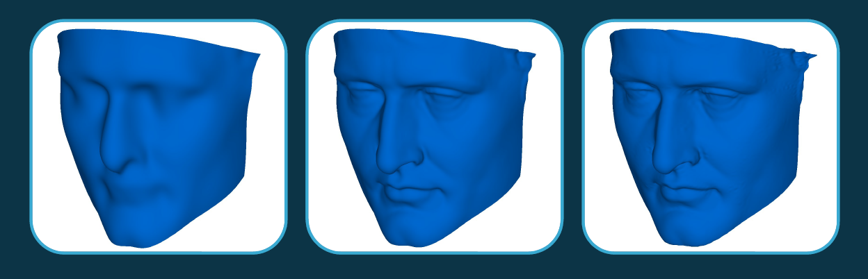
Figure 13
Again, this approach has some limitations. For example, if we try to represent the rabbit with a single surface, the result would be unacceptable. We need a new strategy.
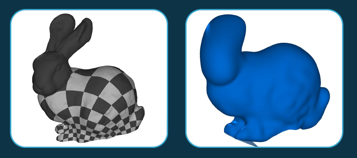
Figure 14
As for the fitting analytic surfaces with the least squares method, there are also some options: the surface type can be explicitly specified, or detected automatically. We can detect and reject outliers with certain criteria, or introduce some kind of shape control to avoid creating nearly degenerate surfaces (e.g., nearly flat or nearly cylindrical cones). The inputs here are also a set of triangles and the expected accuracy. In this case, the accuracy value is used only to verify the result (pass or fail).
The following images are examples of fitting some geometric primitives.
Plane:
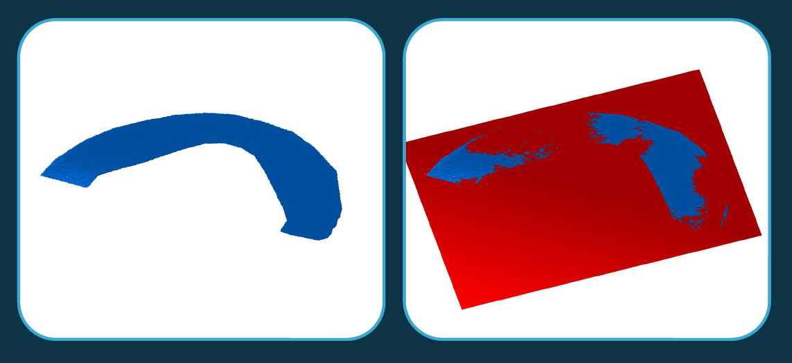
Figure 15
A cylinder fitted to a poor-quality mesh:
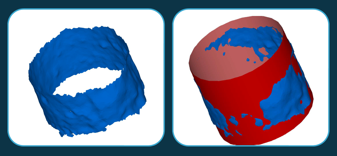
Figure 16
Next, a sector of the cylinder is shown:
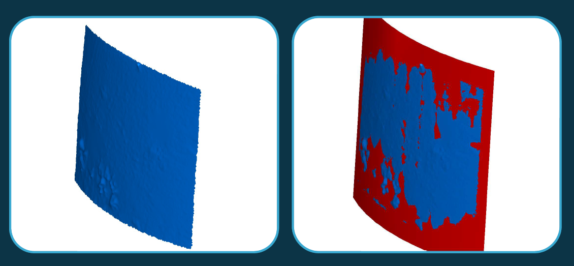
Figure 17
This image explains why we should reject the outliers. Note the artifacts on the bottom left of the mesh. If you consider the artifacts when fitting, they will cause some systematic bias. An outlier rejection module removes such artefacts giving better results.
This image shows a sphere fitting.
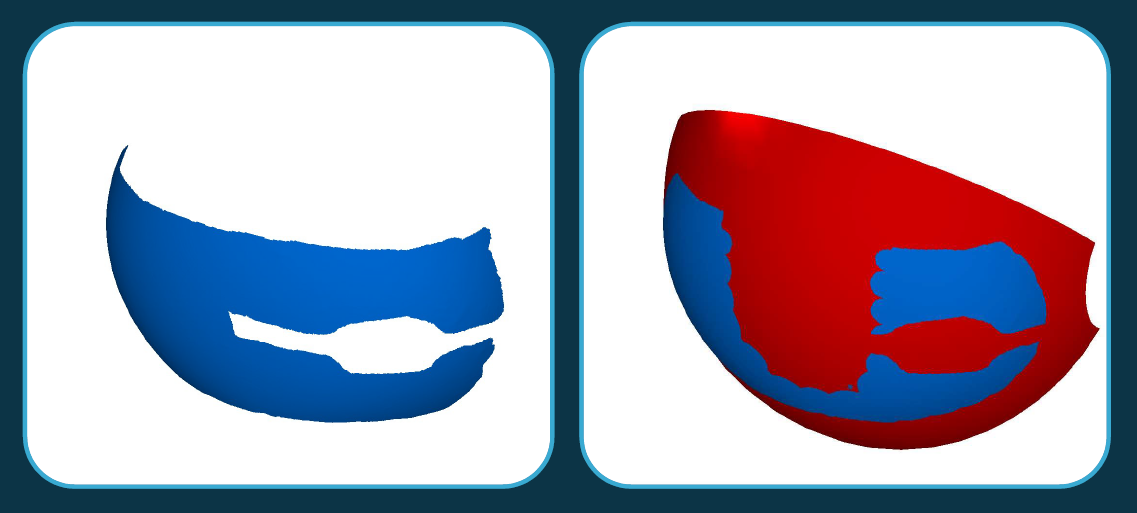
Figure 18
This is a cone.
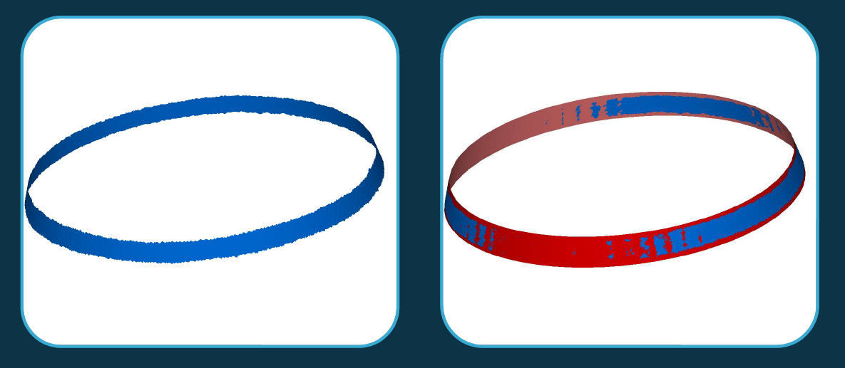
Figure 19
This is a torus.
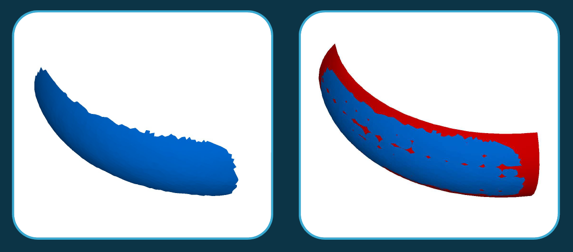
Figure 20
So, all the analytical primitives can be fitted.
A few words about B-Shaper. Its foundations are still the same, but the module has been upgraded. In particular, now it uses a new topology. It has also gotten new fitting algorithms. This has improved the handling of closed surface seams and optimized other processes.
In the future, B-Shaper will have a dedicated functionality for scanned meshes. It is known that any fully automatic algorithm cannot handle such meshes. Another key challenge is the semi-automatic reverse engineering functionality with interactive segmentation and user prompts. The next goal is the detection of kinematic surfaces. So far, the tool recognizes surfaces of rotation, but it needs to be optimized and extended to recognize surfaces of extrusion. An automatic NURBS patches net generation is equally important. This is required to parametrize complex surfaces like the Stanford Rabbit.
The plans for polygonal modeling advancements include surface fitting with constraints. For example, we might need to fit not just a cylinder, but a cylinder with its axis perpendicular to a given plane. There are also plans for the mesh diagnosis and healing tools. Basic healing is usually insufficient. A mesh may have a variety of issues: gaps, holes, self-intersections, topological defects... We need efficient mesh diagnosis and healing tools. In the future, we will detect and align meshes and clouds represented in different coordinate systems. This is important for model comparing, for example. Suppose we have a parametric model of the part and a point cloud from a 3D scanner. We need to align the models and project them onto each other. Our to-do list also includes further enhancement of the Boolean operations adding the algorithms to the API if they are available internally. For example, such algorithms are segmentation by sharp edges, mesh smoothing, or estimation of surface properties like curvature.
The left image shows the principal curvature directions estimated on triangulation, and the right image shows the direction of the normal vectors.
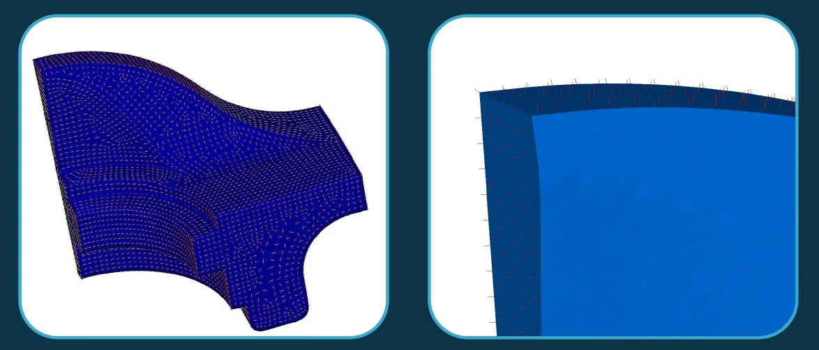
Figure 21

Author:
Alexander Lonin
Team Lead of polygonal modeling, Ph.D.
C3D Labs