In this paper, I present an overview of curve mesh surfaces and the general mathematical concepts behind surface modeling.
Surfaces that are defined by curve meshes are valuable for modeling complex shapes with CAD systems. Such surfaces are created with the assistance of two sets of intersecting curves. These form a matrix-like mesh, and are sometimes is called “generating curves.” The curve mesh surface always passes through these generating curves.
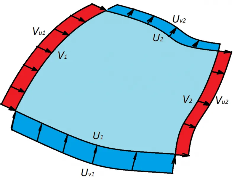
Specifying the derivative values of such curves is a convenient way to meet conditions at the boundaries of the surface. Fig. 1 shows a curve mesh surface in blue defined by two curves in each direction, u and v. The derivative value shown by the arrows is used to create the tangent mattings to the second surface in brown.
The two sets of generating curves define parametric isolines on the resulting surface. The u generating curves define surface isolines with the constant parameter v=const, while the v generating curves define surface isolines with the constant u=const parameter. Each cell (patch) of a curve mesh surface is a Coons face, named after its inventor. The simplified equation is:
The two H terms in Eq. (1) are Hermitian (a square matrix, named after its founder) forms for each direction. Each Hermitian form guarantees that the surface passes through all the transverse generating curves. For example, the cubic Hermitian form in the u direction makes the surface pass through the v curves (Fig. 2).
 Fig. 2. Hermitian form for the u direction making the surface pass through the v curves, with the Hermitian for the v direction making the surface pass through the u curves (see Fig. 3)
The cubic Hermitian forms are given as
where
α1, α2, β1, β2 are Hermitian functions defined over the specified range of parameters
U1(u), U2(u), V1(v), V2(v) are boundary curves of the surface patch
Uv1(u), Uv2(u), Vu1(v), Vu2(v) is the first derivative flux across the patch boundaries
For simplicity, we assume that the boundary curves and the surface have the same parameters. In real life, this is usually not the case, and so we need to reparameterize the original curves. Considering the properties of the Hermite function, it is clear that in addition to passing through the reference curves in the geometric sense, the Hermitian forms also define the transverse vector fluxes at the boundary “flows” of Vu for the v boundaries, and Uv for the u boundaries.
When we cancel the contribution of the Hermitian forms for the first direction to the calculation results at the boundaries for the second direction, a third term is introduced into the Coons face equation. For a cubic form, the term is as follows:
where
Another version considers the coincidence of the surface with the generating curves at the patch boundaries:
In matrix M0 the elements of the first two rows and the first two columns are precisely defined by the generating curves, while the remainder of the elements are mixed derivatives to be defined either as constants, or else as functions of u and v. The choice depends on the form in which the flux functions are defined. I will consider this in detail later.
For now, note the property of the mixed components required to reduce the M(u,v) function with the Hu(u,v) Hermitian form at the u boundaries, and with the Hv(u,v) Hermitian form at the v boundaries. For the v=vmin boundary, this property is expressed as follows, assuming that the elements of the M0 matrix may depend on u and v:
We can verify, with a direct substitution, that it keeps the transverse vector Uv1 on the boundary v=vmin. The same conditions can be deducted for the other boundaries of the patch. To summarize, for any order of differentiation n the Coons shape has the following properties at its boundaries:
The Coons shape can be constructed on Hermitian forms of various degrees, starting with the linear form. It follows that the Hermitian forms may have different orders for the u and v directions. I believe higher-order forms are not required, unless necessary. For example, using a cubic Hermitian form for u is suitable if the surface contains several patches in that direction, or if the first derivative of the transition surface is defined on any of the v boundaries. If neither is available, the linear form is sufficient. The bicubic Hermitian form for u is suitable for smooth (C2-style) transitions between patches along the u direction, or when the second derivative of the transition at the v boundaries is defined:
Flux Function Estimation Methods
With this brief overview of surface properties completed, we can move on to flux function estimation methods (Fig. 4). The flux function can be derived with two options:
1) Interpolating the mesh values between the mesh nodes using the Hermitian equations.
2) By setting directly for the corresponding reference curves.
Note that we did not, so far, study the second option mentioned above. However, this approach has some advantages, although it is more complicated. For example, the flux relationship can be made more flexible in terms of adjusting to surface shapes. It means that more vector values can be specified within the interval, in addition to the mesh nodes. We can estimate these values by, for example, minimizing the curvature-based surface function. The interpolation approach may lead to an unexpectedly warped or ribbed surface, especially as the orders of Hermitian forms increase, or when the generating curves are spaced sparsely. Also, the explicit definition of flux functions solves the issue of specifying the mixed derivatives at the nodes, because now they are estimated directly by the functions themselves.
Now we consider constructing the flux function by mesh interpolation. This is simple. Using the v=vmin boundary as an example, we consider the flux of the vector of the Uv1(u)first derivative. From the Coons face properties, the flux vector at the start and end points of the boundary is equal to the following:
The order of interpolation depends on the degree of the Hermitian form for the u direction. If a linear form is used, then the data is sufficient to deduct a flux function:
For a cubic form, we should specify additional values at the mesh nodes, which have mixed derivatives. In this case, the flux function is expressed as follows:
For a bicubic relationship, another mixed derivative is introduced:
The introduced values are mixed derivatives. They can be directly verified by calculating the corresponding derivatives of Coons face (1) using Eq. (2), (3), and (8-10). As their geometric meaning is known, we can find an approach to produce their definitions. I use the finite difference method. The mixed derivative is calculated with a four-point stencil in some neighborhood of the mesh node based on a lower-order Coons face, which does not require the value of this node parameter. For example, we can find the ruv mixed derivative a surface formed by linear forms; it looks like this:
Constructing the flux function for the second derivative does not differ significantly from the method described above for the first derivative. For the bicubic Hermitian form, it is expressed as follows:
Note that the introduction of higher degree functions makes the calculation very sensitive to the selection of higher mixed derivatives, so it is better to separate the Hermitian forms by their degrees, and then use the lowest orders acceptable for the specific surface.
The flux function can also be used to satisfy a range of boundary conditions. Moreover, this is the most challenging point in curve mesh surface modeling. By boundary conditions, I mean that a curve mesh surface that can be joined to another surface along its boundary curve by a variety of ways. In this case, the boundary should be a curve on the surface.
I will consider tangent and curvature-based transitions; I will not consider the normal-based transition, because it is not fundamentally different from the tangent transition.
Using the same v=vmin boundary as an example, consider the Uv1(u) flux vector. The vector calculated from Eq. (8), (9), or (10) does not satisfy the transition boundary conditions, so a more complex calculation is required. There are two different approaches:
1) The first approach applies constraints to the Uv1(u) flux function
2) The second approach replaces the interpolated object
The first approach interpolates the x, y and z global components of the Uv1(u) vector. The second approach interpolates tangent, normal, and binominal components of the flux vector. Afterwards, they are converted to the global coordinate system. (Note that the tangent component goes along the boundary between the surfaces; the normal component is normal to the transition surface; and the binormal component is perpendicular to the boundary in the tangent plane.) Such an interpolation naturally preserves tangency conditions. Moreover, the interpolation preserves the sign of the binormal component of the flux vector. This is not true for global interpolation, which, in this respect, is more unpredictable.
Let us consider the first approach in greater detail, in which we apply constraints to the flux function. For this approach, the tangency condition is reduced to the exclusion of the normal component from the flux vector:
In addition, this approach restricts the nodal mixed derivatives used in Eq. (9-10) to calculate the Uv1(u) vector. It follows from condition (13) that
This identity also means that all derivatives of this expression concerning u are identical to zero:
It follows that the normal component of the nodal mixed derivative ruv at the boundary shall satisfy the following equality:
The double differentiation of equality (14) produces the constraint applied to the normal component of the mixed derivative ruuv as follows:
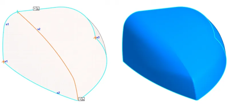
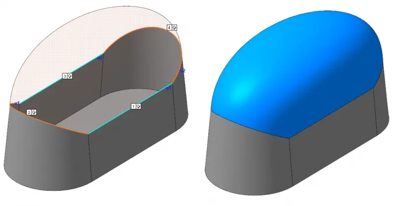
Inequalities (13-15) are the equations needed for calculating the flux function of the first derivative and satisfying the tangent condition. They also define the constraints applied to the mixed derivatives at mesh nodes. Fig. 5 shows the model built with the first derivative-based transition at the two boundaries.
Curvature-based Transition Conditions
Next, I want to consider curvature-based transition conditions. To construct this transition surface, the flux vector of the second derivative (12) is adjusted: its normal component shall have a strictly defined value:
where k is the normal curvature of the surface in the direction of the Uv1(u) vector. The flux vector of the second derivative is represented as two summands: the first one eliminates the normal component from the interpolated vector, and the second one sets the required value for the following component:
Similar to the first derivative case, the nodal mixed derivatives shall satisfy the following conditions:
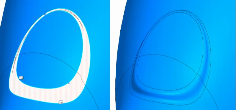
Fig. 6 shows an example of a model built with a curvature-based transition.
The second interpolation method, as I already mentioned, is applied to the vector components in a local coordinate system. In other words, the flux function should be constructed in a local coordinate system. For this (we consider the same v=vminboundary) the rv nodal transverse vectors and their derivatives ruv and ruuv are converted from the global to a local coordinate system.The Hermitian function is constructed from the vectors and their derivatives in a manner similar to Eq. (8-10) with respect to the local basis. The transverse vector and its derivative are converted with the following equation:
where is the transformation matrix,
τ is the tangent vector, n is the normal vector, and b is the binormal at the point.
Another approach is also possible in constructing flux functions within this interpolation method. It may, in some cases, be more practical. In this case, the function construction sequence is reversed.
- First, construct the flux function in the local coordinate system from the flux vector values at the nodes
- Then, using this function, estimate the mixed derivatives at the mesh nodes in the global coordinate system by conversion from the local system
Which Flux Construction Method is Better?
After studying the two flux function construction methods presented here, the reader may have a fair question: Which is better to use? There is no definite answer. There are models in which one method gives significantly worse results than the other one. It seems that we just have to arbitrarily choose one method.
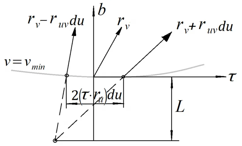
We can, however, take things one step further by introducing a criterion for selecting the most appropriate method for a particular section of the boundary. To do this, consider two closely spaced points on the surface boundary (Fig. 7). The flux vectors reconstructed at these two points intersect at some distance from the boundary. Using the distance, we can estimate the flux function self-intersect trend.
By reducing the distance between two close points, we can represent the criterion in differential form. Skipping the intermediate conversions to save space and time, let us move directly to the result:
This criterion indicates which interpolation method is better suited. The best method gives the longest “self-intersection” distance at the worst point.
The Ambiguity of Mixed Components
Having described the methods for constructing the flux functions for the first and second derivatives, we should reconsider the problem stated at the beginning of the article concerning the conditions imposed on the mixed components in the M(u, v) matrix. It is associated with the ambiguity of the definition of the mixed component at the mesh nodes. Ideally, the derived flux functions for different directions should produce identical derivatives. That is,
If, however, the flux functions for some reason produce different derivatives at the mesh nodes, these equations will not hold. This can happen in the following cases, for example:
1) Two surface boundaries with different mixed derivatives converge at the corner points
2) The mixed derivatives are separated at the surface boundary for any reason
3) The flux functions are defined explicitly, and “do not know anything about each other”
In such cases, there is ambiguity in the selection of the mixed components of the M0 matrix (3) when we consider them as constants that do not depend on u and v. It is possible to avoid this constraint, and maintain the property presented in Eq. (4) by a certain functional representation of the M0 matrix elements.
This representation can be explained using the (umin, vmin) “bottom left” corner of the surface patch as an example. Imagine that the equality is not met for any of the reasons listed above. Then the properties of the Coons face can still be maintained if we find a
M033(u,v) function such that
As example we could look at the following function:
In this case, the Coons face at the v=vmin and v=vmax boundaries are defined by the Hv(u,v) Hermitian form, and at the u=umin and u=umax boundaries by the Hu(u,v) Hermitian form. Because the M0 matrix is now a function of u and v, the estimation of derivatives of the third term in the Coons face (3) is more complicated:
The first summands in Eq. (24) for the M033(u,v) function makes the patch boundary conditions meet, while the second summands at the u=umin and v=vmin boundaries are equal to zero due to the properties of the Hermite functions and their derivatives. So the sum of the flux function values for the first derivative will be maintained. Fig. 8 shows the model with tangent-based transitions at the four surface boundaries.
When the bicubic Hermitian form is used, the second derivatives for the third term of the Coons face should be estimated as follows (3):
Eq. (25) shows that the first terms for the M033(u,v) the function make the boundary conditions meet, while some of the subsequent terms at the u=umin and v=vmin boundaries are equal to zero, due to the properties of the Hermite function and its derivatives. However, Eq. (25) also contains nonzero terms. Fortunately, they can be eliminated if the M033(u,v) function is represented in a slightly different form when the partial derivatives are equal to zero at the corresponding patch boundaries:
It can be seen that this M033(u,v) function turns the partial derivatives at the u=umin and v=vmin boundaries to zero. Then Eq. (26) becomes
It preserves the flux function for the second derivative at the patch boundaries.
Conclusion
This concludes our brief overview of curve mesh surfaces. This paper has presented general concepts behind surface modeling. We omitted some deductions and explanations assuming that the reader has some math background, and with the hope that the reader is curious enough to want to independently compile the missing equations.

Author
Pavel Egorov
Lead Mathematical Programmer of C3D Modeler, C3D Labs


